有时候为了分析深度学习框架的中间层特征,我们需要输出中间层特征进行分析,这里提供一个方法。
(1)输出中间特征层名字
导入所需的库并加载模型
import matplotlib.pyplot as plt
import torch
import torch.nn as nn
from torch.nn import functional as F
from torchvision import transforms
import numpy as np
from PIL import Image
from collections import OrderedDict
import cv2
from models.xxx import Model  # 加载自己的模型, 这里xxx是自己模型名字
import os
device = torch.device('cuda:0')
model = Model().to(device)
print(model)
输出如下,这里我只截取了部分模型中间层输出
Model(
(res): ResNet50(
(conv1): Conv2d(3, 64, kernel_size=(7, 7), stride=(2, 2), padding=(3, 3))
(maxpool): MaxPool2d(kernel_size=3, stride=2, padding=1, dilation=1, ceil_mode=False)
(layer1): Sequential(
(0): ResNet50DownBlock(
(conv1): Conv2d(64, 64, kernel_size=(1, 1), stride=(1, 1))
(bn1): BatchNorm2d(64, eps=1e-05, momentum=0.1, affine=True, track_running_stats=True)
(conv2): Conv2d(64, 64, kernel_size=(3, 3), stride=(1, 1), padding=(1, 1))
(bn2): BatchNorm2d(64, eps=1e-05, momentum=0.1, affine=True, track_running_stats=True)
(conv3): Conv2d(64, 256, kernel_size=(1, 1), stride=(1, 1))
(bn3): BatchNorm2d(256, eps=1e-05, momentum=0.1, affine=True, track_running_stats=True)
(extra): Sequential(
(0): Conv2d(64, 256, kernel_size=(1, 1), stride=(1, 1))
(1): BatchNorm2d(256, eps=1e-05, momentum=0.1, affine=True, track_running_stats=True)
)
)
(1): ResNet50BasicBlock(
(conv1): Conv2d(256, 64, kernel_size=(1, 1), stride=(1, 1))
(bn1): BatchNorm2d(64, eps=1e-05, momentum=0.1, affine=True, track_running_stats=True)
(conv2): Conv2d(64, 64, kernel_size=(3, 3), stride=(1, 1), padding=(1, 1))
(bn2): BatchNorm2d(64, eps=1e-05, momentum=0.1, affine=True, track_running_stats=True)
(conv3): Conv2d(64, 256, kernel_size=(1, 1), stride=(1, 1))
(bn3): BatchNorm2d(256, eps=1e-05, momentum=0.1, affine=True, track_running_stats=True)
)
(2): ResNet50BasicBlock(
(conv1): Conv2d(256, 64, kernel_size=(1, 1), stride=(1, 1))
(bn1): BatchNorm2d(64, eps=1e-05, momentum=0.1, affine=True, track_running_stats=True)
(conv2): Conv2d(64, 64, kernel_size=(3, 3), stride=(1, 1), padding=(1, 1))
(bn2): BatchNorm2d(64, eps=1e-05, momentum=0.1, affine=True, track_running_stats=True)
(conv3): Conv2d(64, 256, kernel_size=(1, 1), stride=(1, 1))
(bn3): BatchNorm2d(256, eps=1e-05, momentum=0.1, affine=True, track_running_stats=True)
)
)
(layer2): Sequential(
(0): ResNet50DownBlock(
(conv1): Conv2d(256, 128, kernel_size=(1, 1), stride=(1, 1))
(bn1): BatchNorm2d(128, eps=1e-05, momentum=0.1, affine=True, track_running_stats=True)
(conv2): Conv2d(128, 128, kernel_size=(3, 3), stride=(2, 2), padding=(1, 1))
(bn2): BatchNorm2d(128, eps=1e-05, momentum=0.1, affine=True, track_running_stats=True)
(conv3): Conv2d(128, 512, kernel_size=(1, 1), stride=(1, 1))
(bn3): BatchNorm2d(512, eps=1e-05, momentum=0.1, affine=True, track_running_stats=True)
(extra): Sequential(
(0): Conv2d(256, 512, kernel_size=(1, 1), stride=(2, 2))
(1): BatchNorm2d(512, eps=1e-05, momentum=0.1, affine=True, track_running_stats=True)
)
)
(1): ResNet50BasicBlock(
(conv1): Conv2d(512, 128, kernel_size=(1, 1), stride=(1, 1))
(bn1): BatchNorm2d(128, eps=1e-05, momentum=0.1, affine=True, track_running_stats=True)
(conv2): Conv2d(128, 128, kernel_size=(3, 3), stride=(1, 1), padding=(1, 1))
(bn2): BatchNorm2d(128, eps=1e-05, momentum=0.1, affine=True, track_running_stats=True)
(conv3): Conv2d(128, 512, kernel_size=(1, 1), stride=(1, 1))
(bn3): BatchNorm2d(512, eps=1e-05, momentum=0.1, affine=True, track_running_stats=True)
)
(2): ResNet50BasicBlock(
(conv1): Conv2d(512, 128, kernel_size=(1, 1), stride=(1, 1))
(bn1): BatchNorm2d(128, eps=1e-05, momentum=0.1, affine=True, track_running_stats=True)
(conv2): Conv2d(128, 128, kernel_size=(3, 3), stride=(1, 1), padding=(1, 1))
(bn2): BatchNorm2d(128, eps=1e-05, momentum=0.1, affine=True, track_running_stats=True)
(conv3): Conv2d(128, 512, kernel_size=(1, 1), stride=(1, 1))
(bn3): BatchNorm2d(512, eps=1e-05, momentum=0.1, affine=True, track_running_stats=True)
)
(3): ResNet50DownBlock(
(conv1): Conv2d(512, 128, kernel_size=(1, 1), stride=(1, 1))
(bn1): BatchNorm2d(128, eps=1e-05, momentum=0.1, affine=True, track_running_stats=True)
(conv2): Conv2d(128, 128, kernel_size=(3, 3), stride=(1, 1), padding=(1, 1))
(bn2): BatchNorm2d(128, eps=1e-05, momentum=0.1, affine=True, track_running_stats=True)
(conv3): Conv2d(128, 512, kernel_size=(1, 1), stride=(1, 1))
(bn3): BatchNorm2d(512, eps=1e-05, momentum=0.1, affine=True, track_running_stats=True)
(extra): Sequential(
(0): Conv2d(512, 512, kernel_size=(1, 1), stride=(1, 1))
(1): BatchNorm2d(512, eps=1e-05, momentum=0.1, affine=True, track_running_stats=True)
)
)
)
(layer3): Sequential(
(0): ResNet50DownBlock(
(conv1): Conv2d(512, 256, kernel_size=(1, 1), stride=(1, 1))
(bn1): BatchNorm2d(256, eps=1e-05, momentum=0.1, affine=True, track_running_stats=True)
(conv2): Conv2d(256, 256, kernel_size=(3, 3), stride=(2, 2), padding=(1, 1))
(bn2): BatchNorm2d(256, eps=1e-05, momentum=0.1, affine=True, track_running_stats=True)
(conv3): Conv2d(256, 1024, kernel_size=(1, 1), stride=(1, 1))
(bn3): BatchNorm2d(1024, eps=1e-05, momentum=0.1, affine=True, track_running_stats=True)
(extra): Sequential(
(0): Conv2d(512, 1024, kernel_size=(1, 1), stride=(2, 2))
(1): BatchNorm2d(1024, eps=1e-05, momentum=0.1, affine=True, track_running_stats=True)
)
)
(1): ResNet50BasicBlock(
(conv1): Conv2d(1024, 256, kernel_size=(1, 1), stride=(1, 1))
(bn1): BatchNorm2d(256, eps=1e-05, momentum=0.1, affine=True, track_running_stats=True)
(conv2): Conv2d(256, 256, kernel_size=(3, 3), stride=(1, 1), padding=(1, 1))
(bn2): BatchNorm2d(256, eps=1e-05, momentum=0.1, affine=True, track_running_stats=True)
(conv3): Conv2d(256, 1024, kernel_size=(1, 1), stride=(1, 1))
(bn3): BatchNorm2d(1024, eps=1e-05, momentum=0.1, affine=True, track_running_stats=True)
)
(2): ResNet50BasicBlock(
(conv1): Conv2d(1024, 256, kernel_size=(1, 1), stride=(1, 1))
(bn1): BatchNorm2d(256, eps=1e-05, momentum=0.1, affine=True, track_running_stats=True)
(conv2): Conv2d(256, 256, kernel_size=(3, 3), stride=(1, 1), padding=(1, 1))
(bn2): BatchNorm2d(256, eps=1e-05, momentum=0.1, affine=True, track_running_stats=True)
(conv3): Conv2d(256, 1024, kernel_size=(1, 1), stride=(1, 1))
(bn3): BatchNorm2d(1024, eps=1e-05, momentum=0.1, affine=True, track_running_stats=True)
)
(3): ResNet50DownBlock(
(conv1): Conv2d(1024, 256, kernel_size=(1, 1), stride=(1, 1))
(bn1): BatchNorm2d(256, eps=1e-05, momentum=0.1, affine=True, track_running_stats=True)
(conv2): Conv2d(256, 256, kernel_size=(3, 3), stride=(1, 1), padding=(1, 1))
(bn2): BatchNorm2d(256, eps=1e-05, momentum=0.1, affine=True, track_running_stats=True)
(conv3): Conv2d(256, 1024, kernel_size=(1, 1), stride=(1, 1))
(bn3): BatchNorm2d(1024, eps=1e-05, momentum=0.1, affine=True, track_running_stats=True)
(extra): Sequential(
(0): Conv2d(1024, 1024, kernel_size=(1, 1), stride=(1, 1))
(1): BatchNorm2d(1024, eps=1e-05, momentum=0.1, affine=True, track_running_stats=True)
)
)
(4): ResNet50DownBlock(
(conv1): Conv2d(1024, 256, kernel_size=(1, 1), stride=(1, 1))
(bn1): BatchNorm2d(256, eps=1e-05, momentum=0.1, affine=True, track_running_stats=True)
(conv2): Conv2d(256, 256, kernel_size=(3, 3), stride=(1, 1), padding=(1, 1))
(bn2): BatchNorm2d(256, eps=1e-05, momentum=0.1, affine=True, track_running_stats=True)
(conv3): Conv2d(256, 1024, kernel_size=(1, 1), stride=(1, 1))
(bn3): BatchNorm2d(1024, eps=1e-05, momentum=0.1, affine=True, track_running_stats=True)
(extra): Sequential(
(0): Conv2d(1024, 1024, kernel_size=(1, 1), stride=(1, 1))
(1): BatchNorm2d(1024, eps=1e-05, momentum=0.1, affine=True, track_running_stats=True)
)
)
(5): ResNet50DownBlock(
(conv1): Conv2d(1024, 256, kernel_size=(1, 1), stride=(1, 1))
(bn1): BatchNorm2d(256, eps=1e-05, momentum=0.1, affine=True, track_running_stats=True)
(conv2): Conv2d(256, 256, kernel_size=(3, 3), stride=(1, 1), padding=(1, 1))
(bn2): BatchNorm2d(256, eps=1e-05, momentum=0.1, affine=True, track_running_stats=True)
(conv3): Conv2d(256, 1024, kernel_size=(1, 1), stride=(1, 1))
(bn3): BatchNorm2d(1024, eps=1e-05, momentum=0.1, affine=True, track_running_stats=True)
(extra): Sequential(
(0): Conv2d(1024, 1024, kernel_size=(1, 1), stride=(1, 1))
(1): BatchNorm2d(1024, eps=1e-05, momentum=0.1, affine=True, track_running_stats=True)
)
)
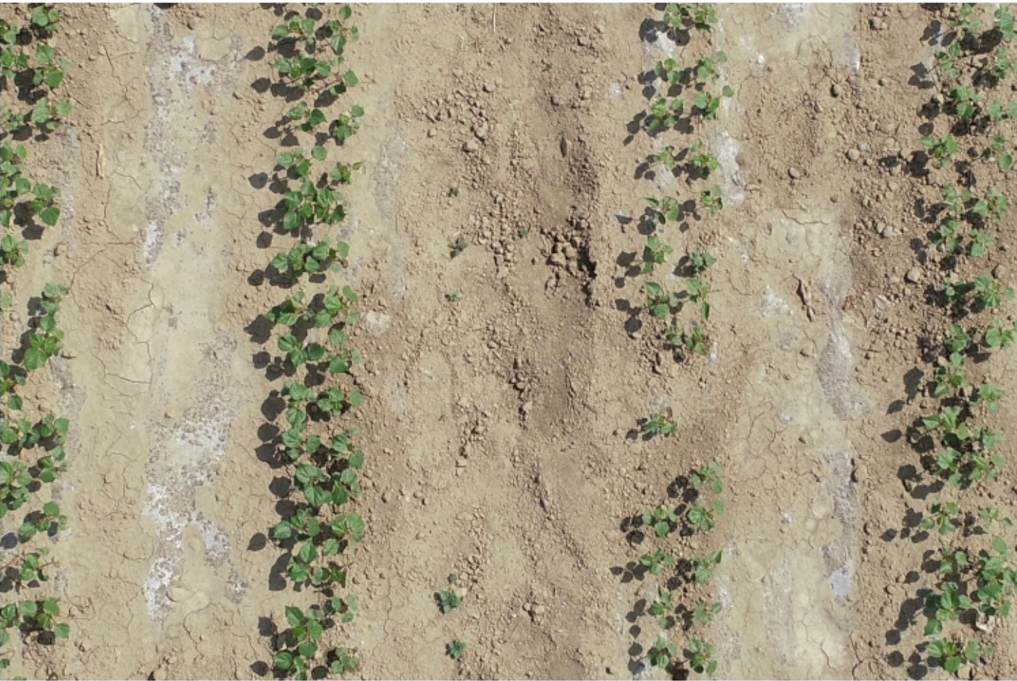
)(2)加载并处理图像
img_path = './dataset//val_data/images/100_0019_0165-11.jpg'
img = Image.open(img_path)
imgarray = np.array(img)/255.0
# plt.figure(figsize=(8, 8))
# plt.imshow(imgarray)
# plt.axis('off')
# plt.show()
加载后如下
将图片处理成模型可以预测的形式
# 处理图像
transform = transforms.Compose([
    transforms.Resize([512, 512]),
    transforms.ToTensor(),
    transforms.Normalize([0.485, 0.456, 0.406], [0.229, 0.224, 0.225])
])
input_img = transform(img).unsqueeze(0)  # unsqueeze(0)用于升维
# print(input_img.shape) # torch.Size([1, 3, 512, 512])(3)可视化中间层
1.定义钩子函数
# 定义钩子函数
activation = {}  # 保存获取的输出
def get_activation(name):
    def hook(model, input, output):
        activation[name] = output.detach()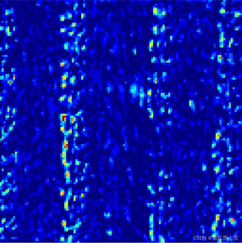
return hook2.可视化中间层特征,这里选择了一个层,其他的自己可以类推
# 可视化中间层特征
checkpoint = torch.load('./checkpoint_best.pth')  # 加载一下权重
model.load_state_dict(checkpoint['model'])
model.eval()
model.res.layer1[2].register_forward_hook(get_activation('bn3'))  #resnet50 layer1中第三个模块的bn3注册钩子
input_img = input_img.to(device)  # cpu数据转一下gpu,这个看你会不会报错,我的不转会报错
_ = model(input_img)
bn3 = activation['bn3']   # 结果将保存在activation字典中  bn3输出<class 'torch.Tensor'>, tensor是无法用plt正常显示的
# print(bn3.shape)  # 调试到这里基本成功了
bn3 = bn3.cpu().numpy() # 转一下numpy,  shape:(1,256, 128, 128)
plt.figure(figsize=(8,8))
plt.imshow(bn3[0][0], cmap='gray')  # bn3[0][0]  shape:(128, 128)
plt.axis('off')
# # shape:(128, 128)
plt.show()可视化结果
(4)利用循环输出多张图像可视化中间层
整合上面的代码,利用循环输出验证集中的多张图像中的可视化中间层
# 加载依赖包
import matplotlib.pyplot as plt
import torch
import torch.nn as nn
from torch.nn import functional as F
from torchvision import transforms
import numpy as np
from PIL import Image
from collections import OrderedDict
import cv2
from models.M_SFANet import Model
import os
import glob
# 定义钩子函数
activation = {} # 保存获取的输出
def get_activation(name):
def hook(model, input, output):
activation[name] = output.detach()
return hook
# 加载模型
device = torch.device('cuda:0')
model = Model().to(device)
checkpoint = torch.load('./checkpoint_best.pth') # 加载一下权重
model.load_state_dict(checkpoint['model'])
model.eval()
model.res.layer1[2].register_forward_hook(get_activation('bn3')) #resnet50 layer1中第三个模块的bn3注册钩子,如果需要其他层数就用其他的
# 利用循环输出多个可视化中间层
#读取需要输出特征的图像
DATA_PATH = f"./val_data/"
img_list = glob.glob(os.path.join(DATA_PATH, "images", "*.jpg")) # image 路径
img_list.sort()
for idx in range(0, len(img_list)):
img_name = img_list[idx].split('/')[-1].split('.')[0] # 获取文件名
img = Image.open(img_list[idx]) # 可以读到图片
imgarray = np.array(img)/255.0
# 处理图像
transform = transforms.Compose([
transforms.Resize([512, 512]),
transforms.ToTensor(),
transforms.Normalize([0.485, 0.456, 0.406], [0.229, 0.224, 0.225])
])
input_img = transform(img).unsqueeze(0) # unsqueeze(0)用于升维
input_img = input_img.to(device) # cpu数据转一下gpu,这个看你会不会报错,我的会报错
_ = model(input_img)
bn3 = activation['bn3'] # 结果将保存在activation字典中 bn3输出<class 'torch.Tensor'>, tensor是无法用plt正常显示的
bn3 = bn3.cpu().numpy()
plt.figure(figsize=(8,8))
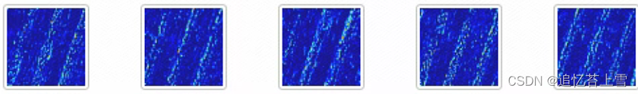
plt.imshow(bn3[0][0], cmap='jet') # bn3[0][0] shape:(128, 128)
plt.axis('off')
# # shape:(128, 128)
plt.savefig('./feature_out/res50/layer1/{}_res50_layer1'.format(img_name), bbox_inches='tight', pad_inches=0.05, dpi=300)保存至文件夹中如下
---------------------------------------------------更新于2023.1121.28 -----------------------------------------
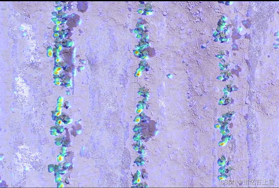
(5)利用循环输出多张图像类激活热力图
使用类激活热力图,能观察模型对图像识别的关键位置。
这里接着上面的获得的特征图进一步得到类激活热力图
接着上面获取到bn3,代码如下
    bn3 = activation['bn3']   # 结果将保存在activation字典中  bn3输出<class 'torch.Tensor'>, tensor是无法用plt正常显示的

    '''
    以下代码用于输出特征图
    bn3 = bn3.cpu().numpy()
    plt.figure(figsize=(8,8))
    plt.imshow(bn3[0][0], cmap='jet')  # bn3[0][0]  shape:(128, 128)
    plt.axis('off')
    # # shape:(128, 128)
    plt.savefig('./feature_out/res50/layer4/{}_res50_layer4'.format(img_name), bbox_inches='tight', pad_inches=0.05, dpi=300)
    '''

    # 将特征图用类热力图形式叠加到原图中
    bn3 = bn3[0][0].cpu().numpy()
    bn3 = np.maximum(bn3, 0)
    bn3 /= np.max(bn3)
    # plt.matshow(bn3)
    # plt.show()

    # img1 = cv2.imread('./dataset/ShanghaiTech/part_A_final/val_data/images/100_0019_0165-11.jpg')
    img1 = cv2.cvtColor(np.asarray(img), cv2.COLOR_RGB2BGR)  # PIL Image转一下cv2

    bn3 = cv2.resize(bn3, (img1.shape[1], img1.shape[0]))
    bn3 = np.uint8(255 * bn3)
    bn3 = cv2.applyColorMap(bn3, cv2.COLORMAP_JET)
    heat_img = cv2.addWeighted(img1, 1, bn3, 0.5, 0)

    cv2.imwrite('./heatmap_out/res50/layer1/{}_res50_layer1.jpg'.format(str(img_name)), heat_img)
输出如下